1. Overview
Take-home Exercise #4: Visualizing and Analyzing Daily Routines
1.1 The Task
In this exercise, we are going to reveal the daily routines of two selected participant of the city of Engagement, Ohio USA.
The data should be processed by using appropriate tidyverse family of packages and the statistical graphics should be prepared using ViSIElse and other appropriate visual analytics methods.
2. Getting Started
2.1 Installing and loading the required libraries
Before we get started, it is important for us to ensure that the required R packages have been installed. For the purpose of the exercise, the tidyverse and ViSiElse packages will be mainly used.
The code chunk below is used to check if the necessary R packages are installed in R. If they have yet, then RStudio will install the missing R package(s). If are already been installed, then they will be loaded in R environment.
packages = c('tidyverse', 'knitr', 'rmarkdown', 'data.table', 'ViSiElse', 'chron', 'lubridate', 'clock')
for(p in packages){
  if(!require(p, character.only = T)){
    install.packages(p)
  }
  library(p, character.only = T)
}
3. Data Import
3.1 Import multiple ParticipantStatusLogs#.csv
In this exercise, all the 72 ParticipantStatusLogs#.csv csv data files in the ActivityLog folder will be used.
The code chunk below imports multiple ParticipantStatusLogs#.csv into R environment by using read_csv() function.
logs <- list.files(path = "data/ActivityLogs/",
                   pattern = "*.csv",
                   full.names = T) %>%
  map_df(~read_csv(.,
                   col_types = cols(.default = "c")))

head(logs)

write_rds(logs, file = 'data/ParticipantStatusLogs_all.rds')
For this exercise, we will be only looking at 2 selected participants i.e. participant ID = 1 and ID = 100. Below code chunk selects the 2 participants and saves the data into local rds file using write_rds() function, which will be used for future processing without reading all the original csv files again.
4. Data Wrangling
4.1 Separate data by participant ID and activity status
Below code chunk first reads the rds file and then further separates the data for the 2 participants individually using filter() function. We also need to separate the different activity status i.e. current mode, hunger status, and sleep status.
logs_only2 <- read_rds("data/ParticipantStatusLogs_only2.rds")

logs_participant1 <- logs_only2 %>%
  filter(`participantId` == "1")

logs_participant100 <- logs_only2 %>%
  filter(`participantId` == "100")


logs_participant1_currentMode <- logs_participant1[c(1:3)]
logs_participant1_hunger <- logs_participant1[c(1:2, 4)]
logs_participant1_sleep <- logs_participant1[c(1:2, 5)]

logs_participant100_currentMode <- logs_participant100[c(1:3)]
logs_participant100_hunger <- logs_participant100[c(1:2, 4)]
logs_participant100_sleep <- logs_participant100[c(1:2, 5)]
4.2 Calculate minutes and transpose the data
Next we are going to calculate the timestamps in minutes of each activity of the day, i.e. the minutes value is the time elapse between the beginning of the day (midnight) and the execution of the activity.
Here we will use ymd_hms() function from lubridate package and times() function from chron package for the calculation of minutes.
The next step is to transpose the data so that activity names will become column names and the minutes will be values in rows. Here we will use group_by() function from dplyr and pivot_wider() function from tidyr package.
It’s also necessary to convert the tibbles to dataframes using as.data.frame() function from base R.
Last but not least, we would like to join the dataframes for all activity status into one dataframe using merge() function.
logs_participant1_currentMode$minutes <- format(ymd_hms(logs_participant1_currentMode$timestamp), "%H:%M:%S")
logs_participant1_currentMode$minutes <- 60 * 24 * as.numeric(times(logs_participant1_currentMode$minutes))

logs_participant1_hunger$minutes <- format(ymd_hms(logs_participant1_hunger$timestamp), "%H:%M:%S")
logs_participant1_hunger$minutes <- 60 * 24 * as.numeric(times(logs_participant1_hunger$minutes))

logs_participant1_sleep$minutes <- format(ymd_hms(logs_participant1_sleep$timestamp), "%H:%M:%S")
logs_participant1_sleep$minutes <- 60 * 24 * as.numeric(times(logs_participant1_sleep$minutes))


p1_currentMode <- logs_participant1_currentMode %>%
  group_by(currentMode) %>%
  pivot_wider(names_from = currentMode, values_from = minutes)


p1_hunger <- logs_participant1_hunger %>%
  group_by(hungerStatus) %>%
  pivot_wider(names_from = hungerStatus, values_from = minutes)


p1_sleep <- logs_participant1_sleep %>%
  group_by(sleepStatus) %>%
  pivot_wider(names_from = sleepStatus, values_from = minutes)


p1_currentMode <- as.data.frame(p1_currentMode)
p1_hunger <- as.data.frame(p1_hunger)
p1_sleep <- as.data.frame(p1_sleep)


p1_allStatus <- merge(p1_currentMode[c(1,3:7)], p1_hunger[c(1,3:7)], by="timestamp")
p1_allStatus <- merge(p1_allStatus, p1_sleep[c(1,3:5)], by="timestamp")
We will repeat the same data wrangling steps for the other participant as well.
logs_participant100_currentMode$minutes <- format(ymd_hms(logs_participant100_currentMode$timestamp), "%H:%M:%S")
logs_participant100_currentMode$minutes <- 60 * 24 * as.numeric(times(logs_participant100_currentMode$minutes))

logs_participant100_hunger$minutes <- format(ymd_hms(logs_participant100_hunger$timestamp), "%H:%M:%S")
logs_participant100_hunger$minutes <- 60 * 24 * as.numeric(times(logs_participant100_hunger$minutes))

logs_participant100_sleep$minutes <- format(ymd_hms(logs_participant100_sleep$timestamp), "%H:%M:%S")
logs_participant100_sleep$minutes <- 60 * 24 * as.numeric(times(logs_participant100_sleep$minutes))


p100_currentMode <- logs_participant100_currentMode %>%
  group_by(currentMode) %>%
  pivot_wider(names_from = currentMode, values_from = minutes)


p100_hunger <- logs_participant100_hunger %>%
  group_by(hungerStatus) %>%
  pivot_wider(names_from = hungerStatus, values_from = minutes)


p100_sleep <- logs_participant100_sleep %>%
  group_by(sleepStatus) %>%
  pivot_wider(names_from = sleepStatus, values_from = minutes)


p100_currentMode <- as.data.frame(p100_currentMode)
p100_hunger <- as.data.frame(p100_hunger)
p100_sleep <- as.data.frame(p100_sleep)


p100_allStatus <- merge(p100_currentMode[c(1,3:7)], p100_hunger[c(1,3:7)], by="timestamp")
p100_allStatus <- merge(p100_allStatus, p100_sleep[c(1,3:5)], by="timestamp")
5. Data Visualization
5.1 Comparing the overall daily routines for the 2 participants
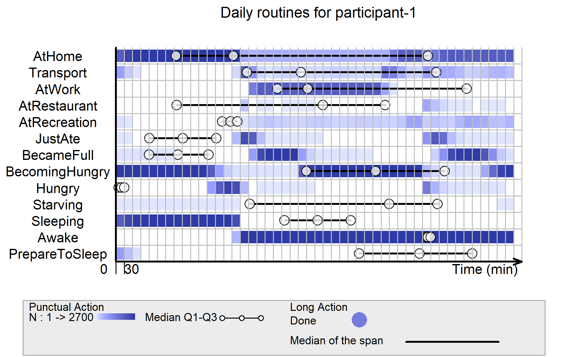
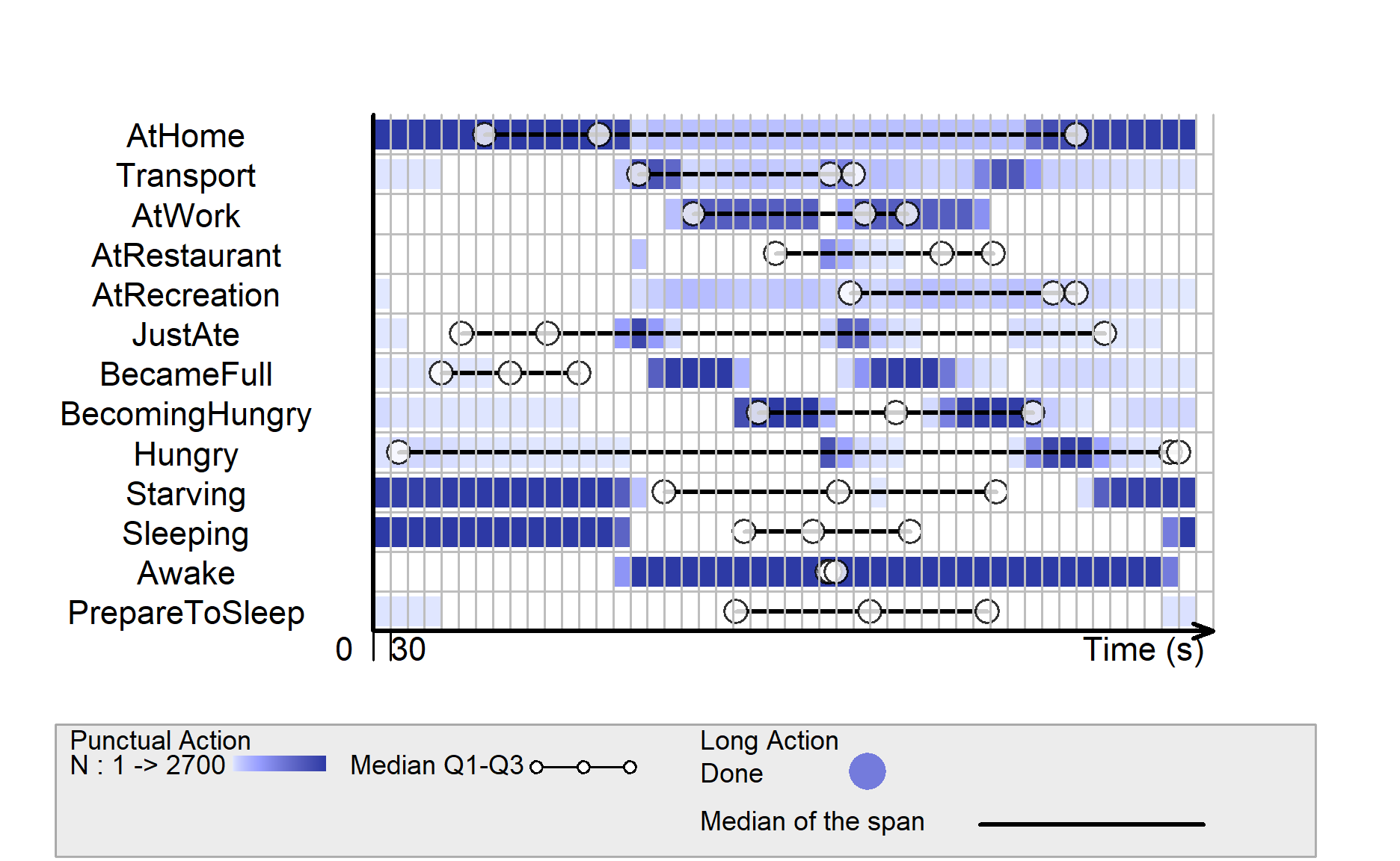
Below code visualizes overall daily life of participant-1 by using ViSiElse package.
It can be seen that participant-1 mostly follows a standard routine from home, transport, work, transport and back to home.
participant-1 usually has 2 meals daily (breakfast and dinner), before work and after work, and it seems that there’s no lunch break during work.
The sleeping behavior of participant-1 is quite consistent, and participant-1 usually prepares to go to bed after midnight.
plot(visielse(p1_allStatus, pixel = 30),
     vp0w = 0.7,
     unit.tps = "min",
     scal.unit.tps = 30,
     main = "Daily routines for participant-1")
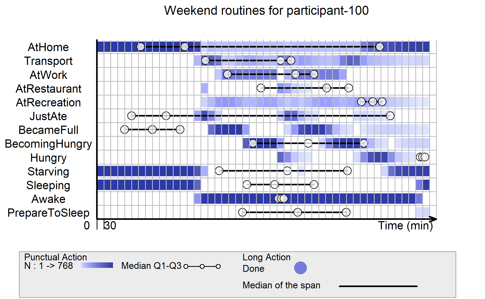
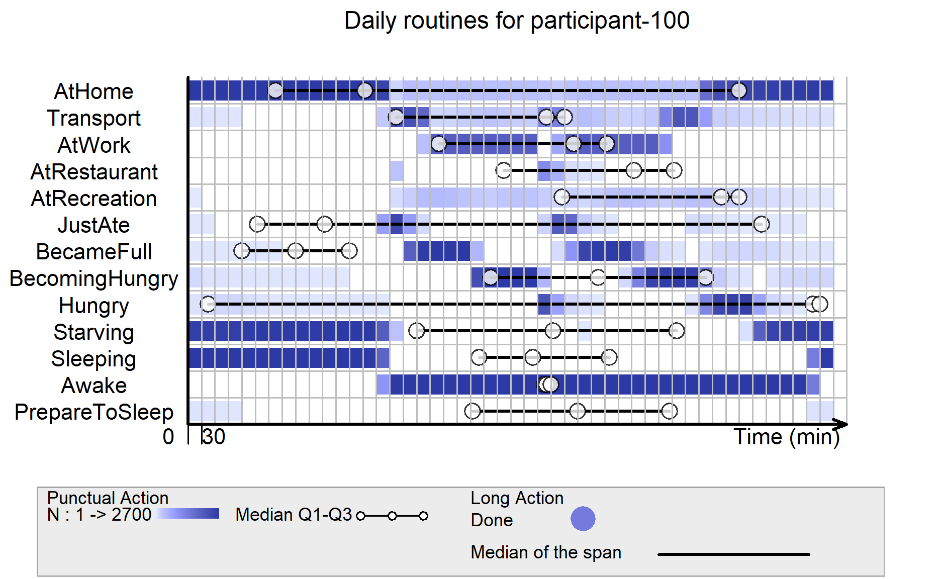
Below code visualizes overall daily life of participant-100.
Comparing to the first participant, participant-100 has a lunch break during day work, and participant-100 usually takes transport to restaurant for lunch during such break.
The 2 main meals of participant-100 are breakfast and lunch only, while participant-100 does not have dinner often.
participant-100 sometimes goes to bed earlier, before midnight, as compared to participant-1.
plot(visielse(p100_allStatus, pixel = 30),
     vp0w = 0.7,
     unit.tps = "min",
     scal.unit.tps = 30,
     main = "Daily routines for participant-100")
5.2 Comparing weekday and weekend routines for each participant
To reveal the differences between weekday life and weekend life, we will calculate the day of the week from the timestamp using wday() function, followed by filtering out the weekday data and weekend data for the 2 participants respectively.
p1_allStatus_days <- p1_allStatus%>%
  mutate(Timestamp = date_time_parse(timestamp, zone="", format = "%Y-%m-%dT%H:%M:%S")) %>%
  mutate(day=wday(Timestamp, week_start=1))

p1_allStatus_weekdays <- p1_allStatus_days%>%
  filter(`day` <=5)
p1_allStatus_weekend <- p1_allStatus_days%>%
  filter(`day`>= 6)


p100_allStatus_days <- p100_allStatus%>%
  mutate(Timestamp = date_time_parse(timestamp, zone="", format = "%Y-%m-%dT%H:%M:%S")) %>%
  mutate(day=wday(Timestamp, week_start=1))

p100_allStatus_weekdays <- p100_allStatus_days%>%
  filter(`day` <=5)
p100_allStatus_weekend <- p100_allStatus_days%>%
  filter(`day`>= 6)
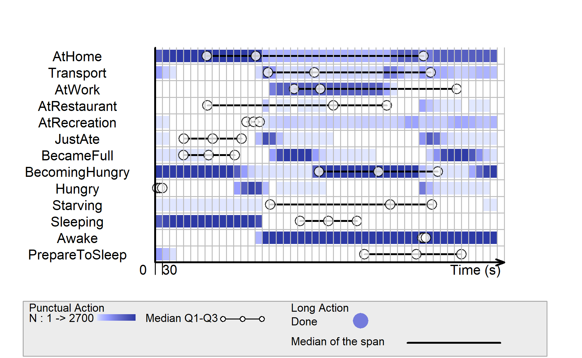
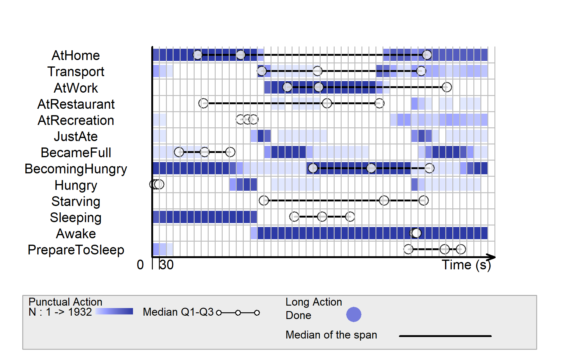
Below code visualizes the Weekday life for participant-1.
We can see participant-1 goes to work during day time and goes to restaurant or recreation in the evening after work. Recreation activity could last until midnight, before participant-1 takes transport back to home.
plot(visielse(p1_allStatus_weekdays[1:14], pixel = 30),
     vp0w = 0.7,
     unit.tps = "min",
     scal.unit.tps = 30,
     main = "Weekday routines for participant-1")
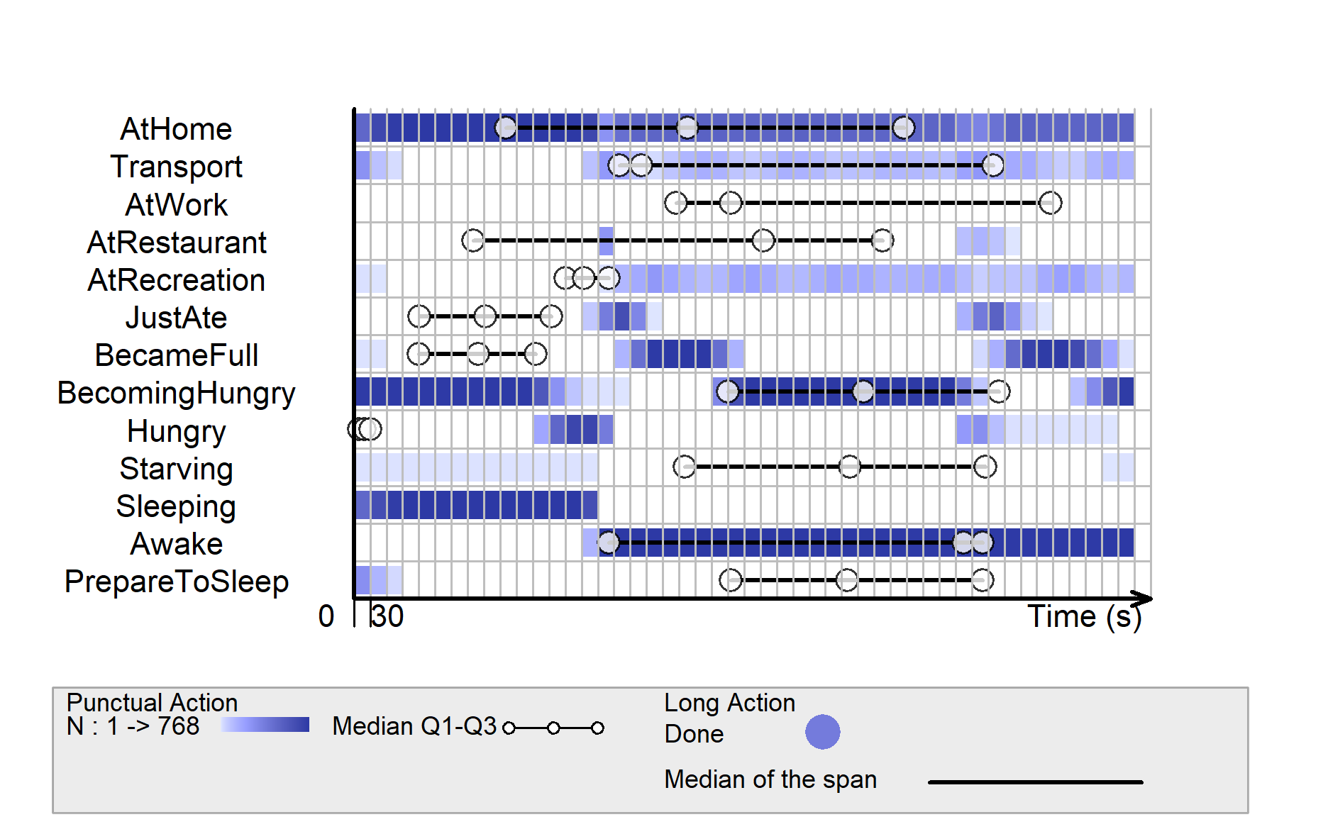
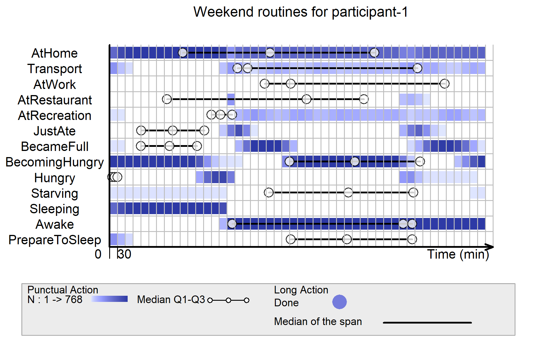
Below code visualizes the weekend life for participant-1.
On weekends, participant-1 does not need to work, so he/she spends most of the time at home or recreation. Even during non-working days, participant-1 still has 2 main meals for breakfast and dinner, without lunch.
plot(visielse(p1_allStatus_weekend[1:14], pixel = 30),
     vp0w = 0.7,
     unit.tps = "min",
     scal.unit.tps = 30,
     main = "Weekend routines for participant-1")
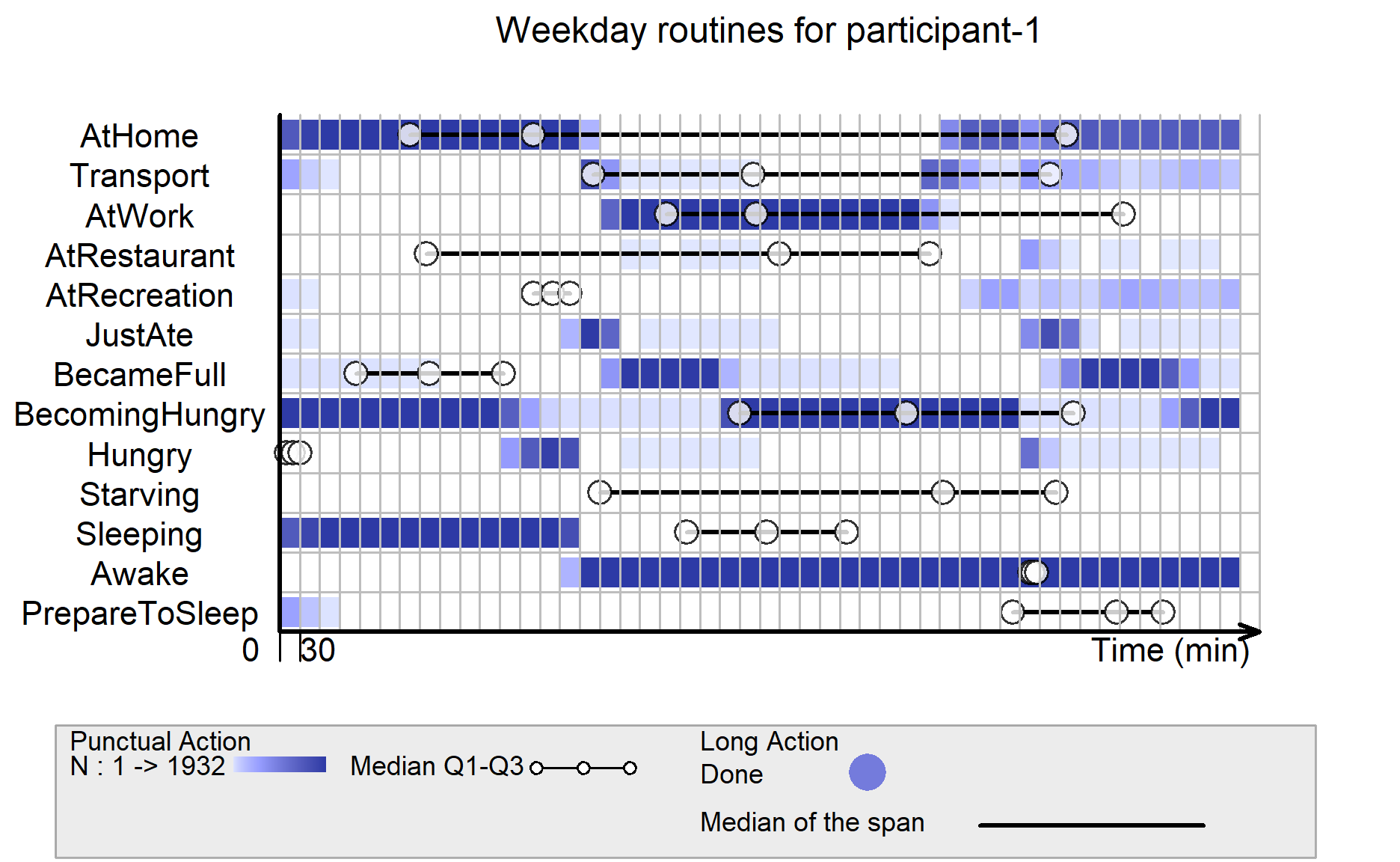
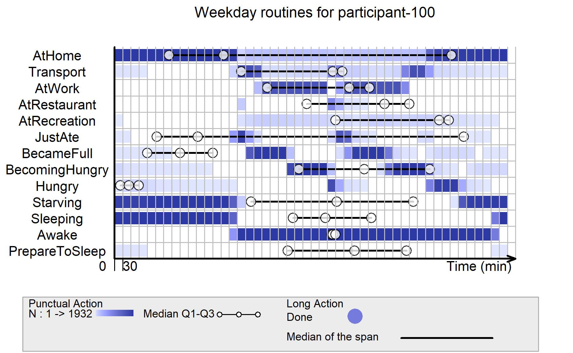
Below code visualizes the weekday life for participant-100.
Even during weekdays, participant-100 sometimes goes to recreation during day time, quite different from participant-1 who mainly stays at work and only goes to recreation in the evening after work.
plot(visielse(p100_allStatus_weekdays[1:14], pixel = 30),
     vp0w = 0.7,
     unit.tps = "min",
     scal.unit.tps = 30,
     main = "Weekday routines for participant-100")
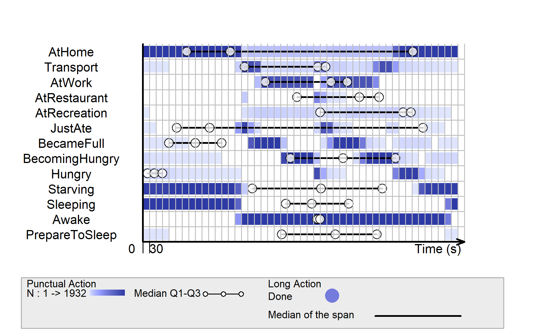
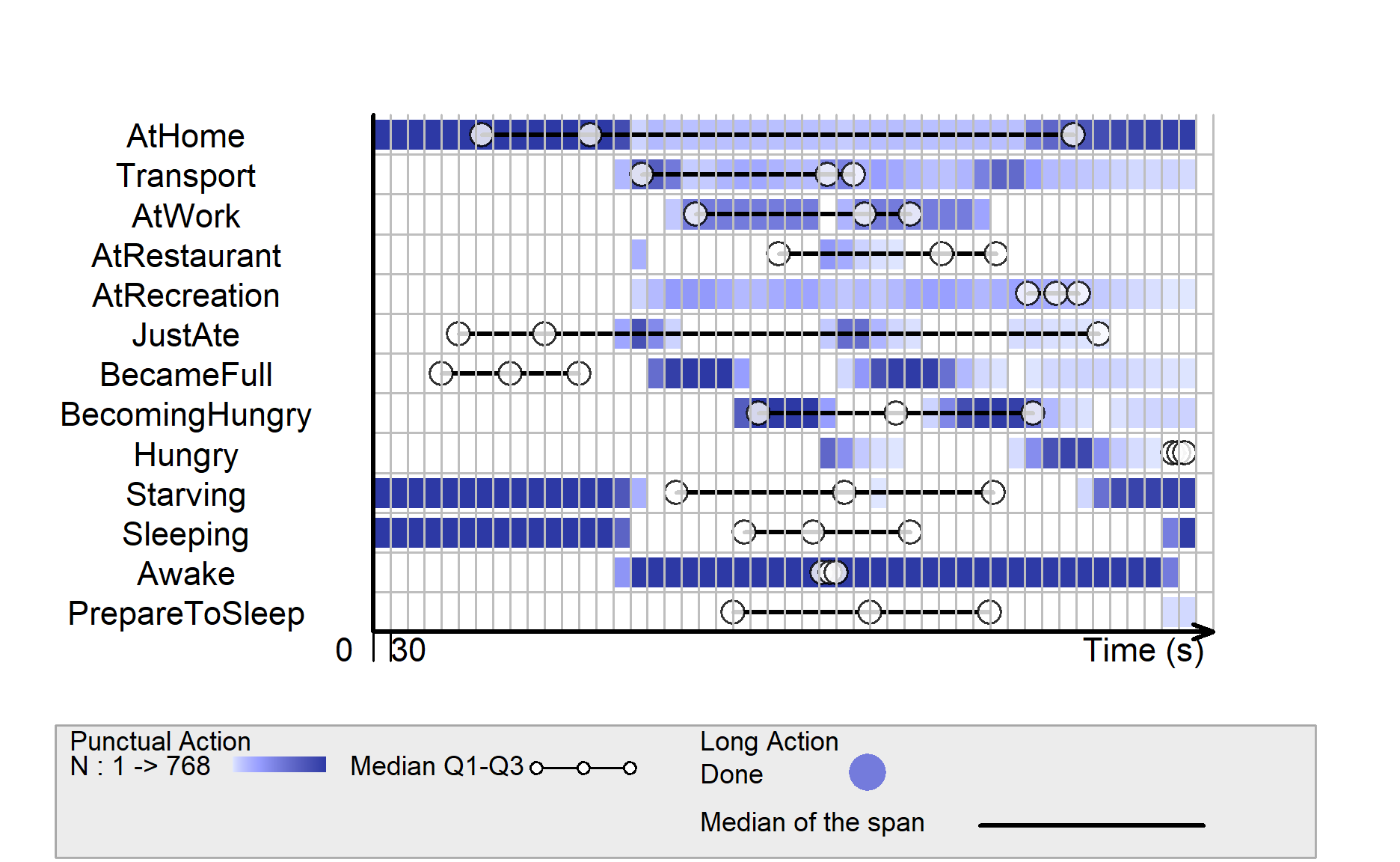
Below code visualizes the weekend life for participant-100.
participant-100 works quite often on weekends, and the life routines on weekend do not have much significant differences from the ones on weekdays.
However, it can be seen that participant-100 only became hungry status only at 2 main time points of the day on weekends, but he/she could be at hungry status across the various timings on weekdays.
participant-100 seems to go to sleep slightly earlier on weekends than weekdays.
plot(visielse(p100_allStatus_weekend[1:14], pixel = 30),
     vp0w = 0.7,
     unit.tps = "min",
     scal.unit.tps = 30,
     main = "Weekend routines for participant-100")